Aperture Synthesis

The signal received from a distant cosmic source is in general a function both of the receivers location as well as of time. If the signal at the observer's plane at any instant is $E(r)$, then spatial correlation function is defined as:

$$\rm {V({\bf x}) = \bigl< E({\bf r}) E^{*}(\bf {r+x}) \bigr>}$$ (2..2)

The function $V$ is referred to as the `visibility function' (or just the `visibility').

In radio interferometry, the visibility function is a complex-valued un-normalized measure of the coherence function of the arriving radiation, modified by the characteristics of the interferometer's antennas. The function ${\mathcal{V}}(u,v)$ of position in the $u$-$v$ plane approximates the Fourier transform of the sky brightness distribution multiplied by the average primary beam pattern of the antennas. This approximation, valid in the limit of small fields of view, is the basis of image formation by aperture synthesis.

For the typical radio array, the relationship between the measured visibility and the source brightness distribution is :

$$\rm {\widetilde{\mathcal{V}}(\it {u,v,w}) = \int {\mathcal{I... ...(\sqrt{1-l^2-m^2} - 1)]}} {{dl\ dm} \over {\sqrt{1-l^2-m^2}}}}$$ (2..3)

The above equation is not a Fourier transform relation between the visibility and the brightness distribution. The visibility is a function of three variables $(u,v,w)$ whereas the brightness distribution is a function of only two variables, $(l \& m)$. For a coplanar array, where a coordinate system can be chosen such as $w=0$, the above relation turns out to be a 2-D Fourier relation.

where $(u,v)$ defines the co-ordinates system of antenna spacings, $(l,m)$ defines cosines in the $(u,v)$ co-ordinates system, ${\mathcal{I}}$ is the source brightness distribution and ${\mathcal{B}}$ is the far field antenna reception pattern.

Correlation of the voltages from any two radio antennas gives the measurement of a single Fourier component of the source brightness distribution. Given sufficient number of measurements of such Fourier components, the source brightness distribution can then be obtained by Fourier inversion. The derived image of the sky is usually called a 'map' in radio astronomy, and the process of producing the image from the visibilities is called as the technique of 'mapping'.

The radio sky (apart from a few rare sources) does not vary for a set of observation. This means that it is not necessary to measure all the Fourier components simultaneously. Thus, for example, one can imagine measuring all required Fourier components with just two antennas, (one of which is mobile), by laboriously moving the second antenna from place to place. This method of gradually building up all the required Fourier components and using them to image the source is called 'aperture synthesis'. If for example one has measured all the Fourier components up to a baseline length of say 25 km, then one could obtain an image of the radio sky with the same resolution as that of a radio-telescope-dish of aperture 25 km, i.e. one has synthesized a 25 km aperture.

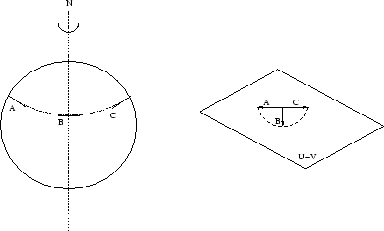
In practice one can use the fact that the Earth rotates to sample the $uv$ plane quite rapidly. As seen from a distant cosmic source, the baseline vector between two antennas on the Earth is continuously changing because of the Earth's rotation (see Figure 2.1). Or equivalently, as the source rises and sets, a range of Fourier components is measured by a given pair of antennas. If one has an array of N antennas spread on the Earth's surface, then at any given instant one measures ${}^NC_2$ Fourier components (or in radio astronomy jargon one has ${}^NC_2$ samples in the $uv$ plane). As the Earth rotates the $uv$ plane gets sampled more and more.

Figure 2.1: The track in the $uv$ plane traced out by an east-west baseline due to the Earth's rotation.

This technique of using the Earth's rotation to improve '$uv$ coverage' was traditionally called `Earth rotation aperture synthesis', but in modern usage, it is usually referred to as `aperture synthesis'. (Ref. Low frequency radio astronomy - J N Chengalur, Y Gupta, Dwarakanath)