Radio Images

Out of 150 sources, 129 source have flat $uv$-distance plots, and are considered as unresolved sources, or in other words, they are a point source for the GMRT array. Two images of such sources are given in the figure 4.3 for reference. All the sources were imaged using AIPS task IMAGR (See chapter 3 for more details) and the images were examined for other sources in the field.

Figure 4.3: Images of the Point Sources at 610 MHz.

The presented figures (see fig. 4.4) are made using the AIPS task KNTR. The parameters used for the task are CLEV=3$\times$; LEVS=-4, -2, -1, 1, 2, 4, 8, 16, 32, 64; DOVECT=0; DOGREY=1; DOCIRCLE=1; PIXRANGE= X Y. CLEV is the absolute value of the level to use an as increment in determining contour levels. Contour levels(n) = CLEV $\times$ LEVS(n). 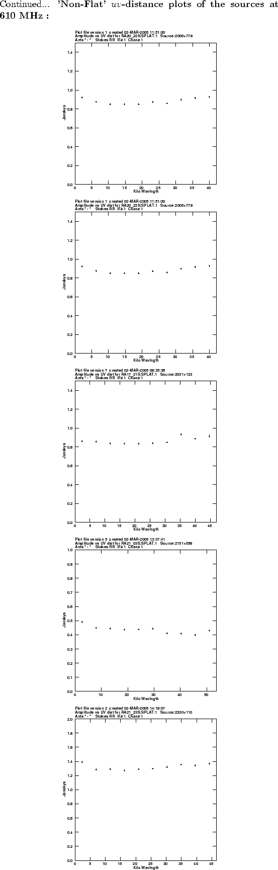CLEV used for most of the map is 3$\times$, where is the $RMS$ of the map (in mJy). LEVS is an array which represent contour intervals. DOGREY is to do a grey-scale image, DOCIRCLE is to extend ticks to form coordinate grid. PIXRANGE is X : the minimum flux density in the image and Y : the maximum flux density in the image.

The contour plots for the 21 sources for which the $uv$-distance plots are non-flat, are shown in the figure 4.4. The $uv$-distance plots of the same sources are also given in the previous section in the figure 4.2. In figure 4.4, the value of CLEV used for the radio images plots for the sources 0303+472 is 3.5$\times$ and for sources 0834+555, 0725-009, 1146+399 is 4$\times$.

Figure 4.4: Images of the sources with non-flat $uv$ plots at 610 MHz.

Figure 4.4: Images of the sources with non-flat $uv$ plots at 610 MHz.

Figure 4.4: Images of the sources with non-flat $uv$ plots at 610 MHz.

Figure 4.4: Images of the sources with non-flat $uv$ plots at 610 MHz.

Figure 4.4: Images of the sources with non-flat $uv$ plots at 610 MHz.

Figure 4.4: Images of the sources with non-flat $uv$ plots at 610 MHz.