Radio Images

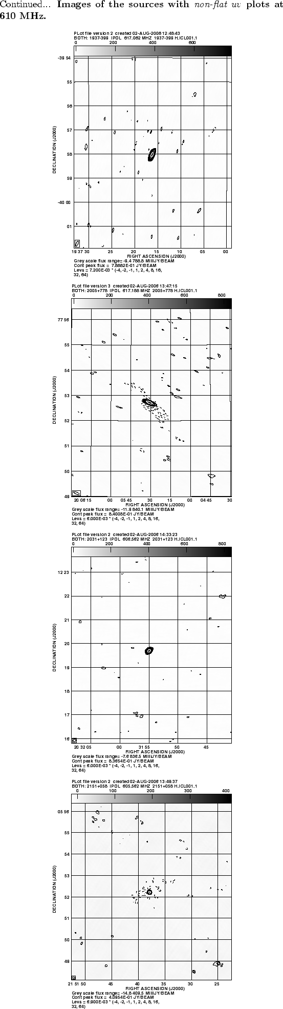
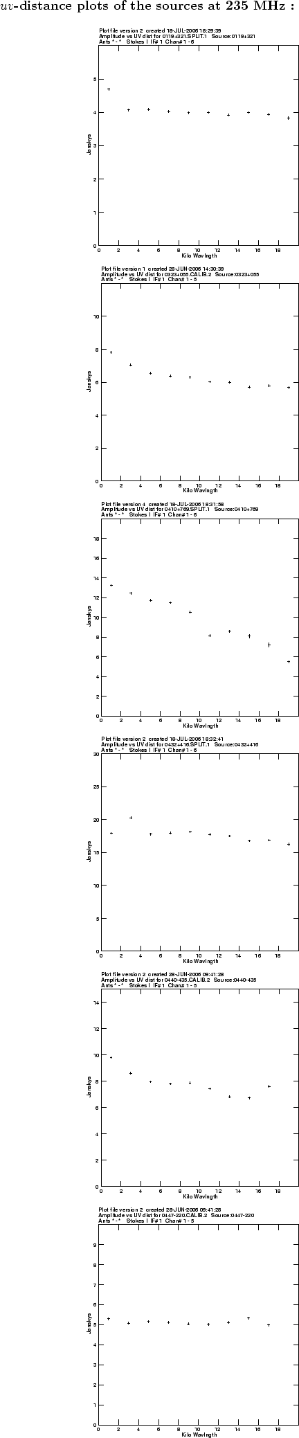
In this section we present 21 contour plots of the sources observed at 235 MHz, for which the flux density (both, the peak surface brightness and the integrated ) is greater than 2.5 Jy. The $uv$-distance plots of the same sources are also presented in the previous section. All the sources were imaged using the AIPS task IMAGR (see chapter 3 for details) and the images were examined for the other sources in the field.

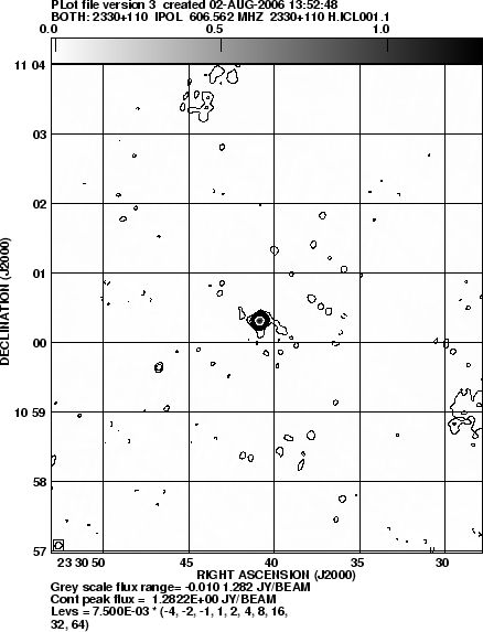
The figure 4.2.2 shows the contour plots of the sources observed at 235 MHz for GMRT. The presented figures are made using the AIPS task KNTR. The parameters used for the task are CLEV=5$\times$; LEVS=-4,-2,-1,1,2,4,8,16,32,64; DOVECT=0; DOGREY=1; DOCIRCLE=1; PIXRANGE= X Y. CLEV is the absolute value of the level to use an as increment in determining contour levels. Contour levels(n) = CLEV $\times$ LEVS(n). CLEV used for most of the map is 5$\times$, where is the $rms$ noise of the map. LEVS is an array which represent contour intervals. DOGREY is to do a grey-scale image, DOCIRCLE is to extend ticks to form coordinate grid. PIXRANGE is X : the minimum flux density of the image and Y : the maximum flux density of the image.

The value of CLEV used for the radio images plots for the sources 0837-198, 1154-350, 0323+055, 0834+555, 0432+416 is 6$\times$, for the sources 1248-199, 1347+122, 1313+675, 1313+675 is 7$\times$ and for the source 1330+251 the value is 8$\times$.

Figure 4.6: Images of the sources at 235 MHz.

Figure 4.6: Images of the sources at 235 MHz.

Figure 4.6: Images of the sources at 235 MHz.

Figure 4.6: Images of the sources at 235 MHz.

Figure 4.6: Images of the sources at 235 MHz.

Figure 4.6: Images of the sources at 235 MHz.