 |
The Fourier Transform (FT) of a signal ![]() is defined as
is defined as
| (8.3.1) |
 |
(8.3.2) |
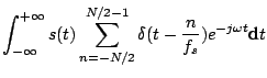
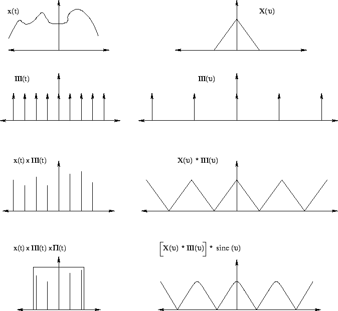
Consider a time series ![]() , which is obtained by sampling a continuous
band limited signal
, which is obtained by sampling a continuous
band limited signal ![]() at a rate
at a rate ![]() (see Fig. 8.3). The
sampling function is a train of delta function III
(see Fig. 8.3). The
sampling function is a train of delta function III![]() . The length of
the series is restricted to
. The length of
the series is restricted to ![]() samples by multiplying with a rectangular
window function
samples by multiplying with a rectangular
window function ![]() . The modification of the signal
. The modification of the signal ![]() due to
these operations and the corresponding changes in the spectrum are shown
in Fig. 8.3. The spectral modifications can be understood from
the properties of Fourier transforms. The FT of the time series can now
be written as a summation (assuming N is even)
due to
these operations and the corresponding changes in the spectrum are shown
in Fig. 8.3. The spectral modifications can be understood from
the properties of Fourier transforms. The FT of the time series can now
be written as a summation (assuming N is even)
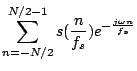
What remains is to quantize the frequency variable. For this the frequency
domain is sampled such that there is no aliasing in the time domain
(see Fig. 8.3). This is satisfied if ![]() =
= ![]() .
Thus Eq. 8.3.3 can be written as
.
Thus Eq. 8.3.3 can be written as
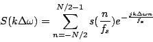 |
(8.3.4) |
Some properties that require attention are:
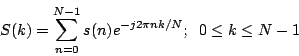
There are several algorithms developed to reduce the number of
operations in the DFT computation, which are called Fast Fourier
Transform (FFT) algorithms. These algorithms reduce the time required
for the computation of the DFT from ![]() to
to ![]() . The
FFT implementation used in the GMRT correlator uses Radix 4 and Radix 2
algorithms.
. The
FFT implementation used in the GMRT correlator uses Radix 4 and Radix 2
algorithms.
In the digital implementation of FFTs the quantization of the
coefficients
![]() degrades the signal to noise ratio
the of spectrum. This degradation is in addition to the quantization
noise introduced by the quantizer. Thus the dynamic range reduces
further due to coefficient quantization. Coefficient quantization can
also produce systematics in the computed spectrum. This effect also
depends on the statistics of the input signal, and in general can
be reduced only by using a larger number of bits for coefficient
representation.
degrades the signal to noise ratio
the of spectrum. This degradation is in addition to the quantization
noise introduced by the quantizer. Thus the dynamic range reduces
further due to coefficient quantization. Coefficient quantization can
also produce systematics in the computed spectrum. This effect also
depends on the statistics of the input signal, and in general can
be reduced only by using a larger number of bits for coefficient
representation.